A round track
We used a meter stick as a way to think about the abstract idea of a number line. We think of a meter stick as a good way to measure things that are straight. But not everything is straight. For example, I like to run around a track. Tracks usually have curves in order to finish at the same place as you start. The shape of most tracks is oval, but let's assume the track is a perfect circle since our focus in this section is circles.
Just like you think of a meter stick as a way to measure distances, I want you to think about this round track as a way to measure distances. The only difference is the meter stick measures distances that go on a straight line but the round track measures distances that go on a curved line in the shape of a circle. In the end, a number line and a circle both contain a line for measuring distances.
I mentioned we have the freedom to invent math. Here, I am inventing a math term. Think of this circle as a number circle, similar to a number line, just round. Of course, my recasting a circle as a “number circle” doesn’t change any of the characteristics of a circle. But it is just my way of viewing a circle from a different perspective. Thinking of a circle as a number circle shouldn’t be difficult because we know the distance around most tracks. For example, a 400-meter track is round (again, assume a circle) and measures 400 meters.
Using the number circle
Once we perceive the number circle as something that can measure round distances, we have several options for what to do next. A logical next step is to identify our perspective of the circle.
In the real world, I’m thinking of a track and would ask, “Where do I want to sit?” I could sit outside the circle like a spectator or at the starting point like a runner. Let’s choose a position a coach may consider and that is to sit in the center of the track, which is the center of our circle. This position has its advantages because I can see everything equally well. Also, the center has a nice symmetry to it, and we (math people) get excited when we encounter symmetry.
Perhaps a second thing to think about is a unit of measurement. We could say 1 represents a distance around the circle, or a distance halfway around the circle. We could even say 1 is the distance across the circle. All these are fine and dandy. But, since I’m sitting in the center of the circle and the entire circle is the exact same distance from where I’m at, it seems only natural to define 1 unit as the distance from the center to any point on the circle. There is nothing right or wrong with this choice. But it will have the advantage of removing clutter later, and removing clutter is the next thing that gets math people excited.
In summary, we have our new “invention” of a number circle where we define the distance from the center to any part of the circle as 1. We give a name to this distance and call it the radius of the circle.
Of course, this number circle isn’t a new invention because what we’re talking about has been around for a long time. Math people call it a unit circle. If you think of a unit as 1, then the name unit circle makes sense since it has a radius 1. We will use this circle often, so you can think of it as either a unit circle or a number circle. Regardless of the label, think of it as a way to measure distance, just like a number line can measure distance around the circle.
Actually, math people define a circle as something that is one-dimensional, just like a number line. It is easy to incorrectly think of the circle as two-dimensional because of the area within a circle. The area within a circle involves two dimensions. But, the circle itself, the track we run on, has only one dimension.
Good. We’re making progress.
Now, we can begin measuring things on this circle. Let’s start easy. What is the distance across the circle? By going across the circle, I refer to traveling from one point on the circle on a straight line to another point on the circle by going through the center of a circle. That distance is just two times the distance from the center to the circle. Since the distance from the center to the number circle is 1, the distance from point to point is 2, and we refer to this as the diameter of the circle.
Then, the next thing that logically comes to mind is the distance around the circle. We should feel like the distance around a circle is similar to a distance across the circle, it’s just one is straight and the other isn’t. A long time ago, the distance around the circle was approximated to be 3.14 times the distance across the circle. We can’t nail this number down exactly but, as of January 2020, we know this number up to 5 times decimal places. That’s 5 followed by 13 zeroes. Rather than writing that many digits, it is easier to call it . That means the distance around a circle is always times the distance across a circle, regardless of the size of the circle. Thus, for our number circle that has a radius of 1 and a distance across of 2, the distance around is and the distance halfway around is half this distance, or .
Have you ever considered how wonderful it is that every circle has this property? There doesn’t seem to be any rational reason for this to be true. It just is. Can you imagine what it would have felt like to be the first person to recognize that the distance around a circle is always , where r is the radius for any circle? This is something simple and profound.
π
What actually is this number we call ? Does have a place on the number line of real numbers? Is she invited to the real (number) party? Yes, she is. This shouldn’t be a surprise since the number circle is like a number line. If we flattened a half circle from our number circle into a straight line, then it would become part of our traditional real number line and would be the distance from the beginning of the half circle to the end of the half circle. We will uncover interesting gems about how relates to a circle later in our journey together.
Recall the real number line consists of two sets of numbers: rational and irrational. Which set would you guess belongs? belongs to the irrational numbers. You may have known this fact. But if you did not know it, you may have guessed is irrational if you knew that the number of digits of continue forever and never repeat. Remember that is one characteristic of an irrational number.
Thus, , you can say, was born in a circle. However, she has wandered around not only in the math world but also in the physical world, and she appears in strange places.
My wife has a heart to help people and an eye for finding someone in need. When she sees a need, she’s often quick to be there to help in whatever way she can. She shows up in unexpected places.
is a lot like that in math. will see a need and it will show up, often in the strangest of places. But must follow a simple principle. Because originated from a circle, there must be a circle somewhere in the problem for to help.
I’ve seen in formulas in actuarial science, for example. But I don’t study circles in actuarial science. So how does get there? There is a circle in the problem somewhere. It’s a great mystery waiting to be solved. Sometimes the circle is obvious, but other times it is not. Finding in an unexpected solution is one of the surprises of math. We will encounter many surprises in math stories. I often will provide some technical details so you can fully appreciate how the pieces fit together. However, you may gloss over some of the technical details if you are primarily interested in the essence of the story. Here is an interesting example of how appears when we least expect it.
Buffon's needle
This story about is based on the work done by the French mathematician Comte de Buffon (1707−1788). Buffon used a technique commonly used today by actuaries and other professionals called the Monte Carlo approach, which is an interesting way to determine probabilities. Buffon’s discovery was shortly after Abraham de Moivre (1667−1754) established probability on solid footing with the first textbook on probability. This problem definitely has interesting history behind it. Here’s Buffon’s problem.
Let’s pretend we have a floor divided by parallel lines that are evenly spaced and the distance between the parallel lines is 2 (inches, centimeters, whatever). Gather 100 toothpicks (or matches) such that their lengths are ½ the distance between the lines. That would be length 1 in our example.
Now we are ready for our experiment. Drop all 100 toothpicks so that they fall randomly on the floor. After all the toothpicks have randomly landed on the floor, identify the picks that touch one of the lines. You can likely anticipate some will be touching a line, but some won’t because the picks are only length 1 and the lines are 2 apart and the picks will fall at different positions. Once you have identified the picks that touch a line, count the number in this group. Let’s assume the number that touch a line is . We know will be an integer between 0 and 100. If none of the picks touch a line, is 0 and if all the picks touch a line, is 100. The likely option is will be more than 0 but less than 100.
If you had nothing better to do, you could perform this experiment 1000 times and record the result. You may ask, “What is the average number of picks I should expect to touch a line?” You would discover, on average, the number of picks that touch a line is about 32. This is about a success rate if we consider the event of touching a line a success. Rather than doing 1000 experiments, can we use math to arrive at an answer?
One way we can consider this question is to ponder how many picks, on average, we need to drop before we expect one pick to touch a line. We’ve actually answered that question by recognizing that about 1 out of 3 picks will touch a line. That means we need to drop about 3 picks before we expect 1 to touch a line.
However, 3 is only an approximate answer. Is there an exact answer? Actually, there is an exact answer and, surprisingly, the exact answer is . Did that answer come out of the blue? Why would the result be exactly ? What we’re saying is if we dropped 314 picks, we would expect 100 to touch a line.
Finding the circle
OK, mystery fans, where is the circle here? arrived, rather unexpectedly, seemingly uninvited. She always brings a circle with her. But our lines are straight, even parallel. Our toothpicks are straight. There are no curves visible in this problem. What brings to the party? Isn’t this interesting? On the surface, everything appears to be straight, but there is a circle hiding somewhere.
In order to understand how arrives, let’s think about how we can solve this. My initial feeling is this problem is impossible to solve. I can picture all the different ways the picks can land and each option appears equally likely. How can I possibly count all the possibilities?
However, the rule in math is when stuck, consider a different perspective. What is another perspective? One perspective is that rather than calculating the exact answer, which appears quite difficult, try to estimate the result. I don’t want just any estimate; I want to find the best estimate. Being able to identify good estimates in math problems is a skill that has tremendous value. Math people are always estimating solutions to problems. If nothing else, the estimate identifies what could be a reasonable result.
How a pick may land appears vague, so let’s try to organize the process of dropping one pick as a sequence of events. Think about the process of a pick landing. One way to think about it is to consider one end of the pick and declare that this end will land first. One end landing is our first event. Then, after one end lands, our second event is the other end lands. Now we have only two events, and thus two things to think about rather than an infinite number of random ways a pick could land. This different perspective is a key pivot in our thinking.
For our first event, how could one end of the pick land? Let’s assume the lines are vertical and they extend as long up and down as needed. Because we assume the lines are infinitely long, then it doesn’t matter where the end lands top to bottom. The important thing is where the end lands in relation to the lines. Let’s consider extreme values. What is the closest an end could land? The end could land right on the line, and the distance would be 0.
What is the farthest an end could land from a line? The farthest it could land from any line is 1. Notice the lines are a distance 2 apart so if the end landed 1.5 from one line, then it would be only 0.5 away from another line. Thus, the farthest distance an end could land from a line is if one end lands exactly halfway between two lines which is a distance 1.
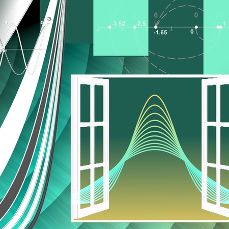
You can observe this from the animated graph above. Think of the vertical lines at and . The point moves between and . When it travels between and , then it is in the red zone which is closest to the line . From to , it is in the yellow zone and it is closest to the line . From to , it is in the teal zone and it is closest to the line . From to , it is in the orange zone and it is closest to the line . However, at any time, the distance of the point to the closest line is somewhere between 0 and 1.
Now we have a range from 0 to 1 for the distance between a pick’s landing point and the closest line to it. We just learned that there are an infinite number of real numbers between 0 and 1 so we must consider all these possibilities and the likelihood, or probability, of landing on each of these numbers.
First, let’s tackle the probability. Would you agree that it seems that any number between 0 and 1 is equally likely to be the distance we are looking for? If one number was more likely than another, then that would be a good point to consider. Since each number is equally likely, it seems like choosing an average distance would be best.
We could assume an extreme value such as 0.99 or 0.01. But, since each number is equally likely, for me, the best guess for the single point estimate is the midpoint between 0 and 1. Therefore, we are assuming for the first event that one end lands a distance exactly from one of the lines. Again, it may seem odd that our “average point” is a distance from one line and a distance to the next closest line. Remember our goal, though, is not to find an average point between two lines. This would be a point halfway between the two lines. Rather, our goal is to choose a point that is an average distance to the closest line. Since the potential distances are from 0 to 1 and each point within this range is equally likely, a reasonable estimate is a point that is a distance 0.5 from a line. In the graph below, the point is a distance of 0.5 to the dotted line. Good. The first end of the pick has landed exactly at 0.5 distance to the next closest line.
Now we are ready to consider the second event. Given this scenario, what is the probability the pick crosses a line after the second end lands?
With one end fixed, think about the possibilities for the second end. How would you describe the possibilities? Notice with one end fixed, we identify the possibilities for where the second end lands by rotating the pick around. An interesting observation is we identified the first end to be within an interval of on a number line and the second end is based on a rotation from 0 to 360 degrees around the first end. Thus, hidden in this experiment is a random process that occurs on a line segment and a random process that involves a rotation that creates a circle. Forward motion and rotational motion are two primary types of motion we experience in our physical world. These are the interesting observations we discover as we consider something so simple as dropping a pick on a floor.
If we think about the rotation of the second end, you can think about this rotation like a hand on a clock. One end of the hand is fixed in the middle of the clock and the other end rotates around. It is this rotation that creates a circle. Are you starting to see where may appear? We don’t know exactly how appears, but now we have found our circle!
Estimating our probability
Given this single scenario, can we identify the probability? Notice if the pick rotates in any part of the shaded area in the graph (Figure 4), the pick intersects the line. If it rotates outside the shaded region, then it does not cross the line.
We now have a good intuition about how this problem works. Remember, we have assumed that the pick’s first end is exactly 0.5 from the closest line. But you should feel comfortable that this midpoint is a good estimate. For this one scenario, can we calculate the probability that the second end lies within the shaded region?
We can view this circle as a normal clock with 12 numbers for each hour. If we worked through the math, we would find that the gray area starts at 1 o’clock and ends at 5 o’clock. That means it covers 4 out of 12 numbers. As a result, our estimate is or .
Wasn’t that slick? The difficulty in arriving at this estimate was not the math but in presenting the dropping of a pick as two events and recognizing what occurs in each event. Really, the only challenging math I skipped was understanding why the gray area starts at 1 o’clock and ends at 5 o’clock.
Some of you may be interested in our clock math, so let’s review the details. The details require some basic trigonometry. Even if you have not had trigonometry or it is rusty, I encourage you to try to understand the math and give it your best shot.
If we consider the shaded area, note that we do not need to calculate the area of the shaded region. What we need is the percentage of the circle that is shaded relative to the entire circle. Notice once we know the percentage of the circle that is shaded, then that percentage equals the probability we want since each rotation is equally likely. In other words, we only need to know what part of the circle is shaded but not its area. This is what makes us think about the angle that exists in the shaded area based on the center of the circle. Since we know there are 360 degrees for a complete rotation, if we have the angle measurement, then we can divide it by 360 to identify what part of the circle is shaded.
Since we are hunting for an angle, maybe we can ignore the entire circle and use a triangle to determine our angle. In other words, we can use the dashed line as a way to create a triangle that still captures the angle we care about. This seems like a good idea because we are used to measuring angles with triangles. This is another common creative math move. The current problem is in the form of a part of a circle. But, since we only care about the angle, we can dismiss the circle, create a triangle, and move to another area of math that specializes with angles. That specialized part of math is trigonometry.
If we are fresh on our trigonometry, we remember there were a lot of ways to calculate angle measurements by using a right triangle. The triangle we created is not a right triangle. But just because a right triangle isn’t here doesn’t mean we can’t find one. Again, symmetry comes to our rescue as we have a clock with one hand pointing to 1 and another to 5. If we insert another hand pointing at 3, we now have 2 triangles rather than 1. Because of the symmetry, we have created two triangles which are mirror images of each other. That means we created two right triangles because we divided a line into two equal parts which creates two 90-degree angles. Thus, we can just focus on one triangle, the top one, and we recognize that it is a right triangle.
What else do we know about this triangle? The hypotenuse is 1 because it is the length of our pick which creates the radius of the circle. The bottom side is 0.5 because we assumed one end of the pick is 0.5 away from the closest line. From trigonometry, we know that if the hypotenuse is 1 and a side is 0.5 for a right triangle, then the triangle is a triangle. We also know the larger angle, , corresponds to the shorter side, which is 0.5. As a result, the angle we care about for this triangle is . This is only half the angle we want. We have an exact copy of the triangle on the bottom, only flipped. Thus, the total angle measurement is . Since a circle has a total of , the shaded region is or . This is a more formal way to arrive at the same result when we simply considered the circle with hands at 1 o’clock and 5 o’clock.
Thus, using a one-point estimate for where the first end lands, we can conclude the probability that the pick crosses a line is . If you just review this picture, doesn’t the result make sense? Maybe your trigonometry isn’t fresh enough to calculate it as , but you should see how this picture captures our estimated result and an estimate of fits a reasonable view of the picture. If we consider all the points from 0 to 1, recall the precise answer is . Since π is about 3.14, our probability estimate of , derived only by using the midpoint, is quite close to the exact probability, which is . That was some interesting math, for sure. As interesting as the math was, what is more interesting is the bigger picture of what we just did.
Reflecting on the experiment
If we choose our best guess of where the first end lands, we get a good answer that we can quantify exactly as . But, if we want the full spectrum of possibilities, the full space that life has to offer, the entire space between the two lines, then we must call on to give us the exact result. I find this to be another trait of . Not only does it show up, but it shows up with beauty!
Let’s take a moment and reflect on the difference between our estimate and the exact answer. Our estimate chose one point within the interval from 0 to 1. Of course, we could estimate with 2 points and perhaps take the average of the two. For example, one point could be the distance and the other point could be . Regardless of which points we choose, or how many points we choose, we are choosing a finite number of points within this interval when we estimate the result.
But what does an exact solution require? An exact solution requires considering every single point within this interval because any point is possible. Now recall our previous journey through the number line. We identified an infinite number of rational numbers within this interval and even a bigger infinite number of irrational numbers. Wouldn’t that indicate that the exact solution cannot solve the problem by reviewing different points, which are things we count? Rather, the exact solution must consider the entire segment from 0 to 1. Do you grasp our dilemma? We cannot answer this question exactly if we remain in a finite world of things we count. In order to solve our math problem, we must exit this finite world and step into a new world.
How can we enter this new world that deals with segments that contain infinite points? This is the world of calculus. Calculus is like the world of Narnia. It’s a world where we do things using techniques that are different from counting. It’s a world that considers the entire spectrum of infinite possibilities and returns an exact result. One would think that through this complicated process our result would be something complicated. Isn’t that the way our real world works? If we bring more cooks into the kitchen, it only adds to the complexity. Of course, a result that contains retains a little mystery because it contains an infinite number of digits. But don’t lose sight that the exact answer to our pick dropping question exactly equals a result that has an infinite number of digits.
You may be curious about this calculus solution. I’m not sharing the calculus solution here. But as we journey further into Lazarus Math, we will learn some tricks from calculus that will make the exact solution to this problem relatively easy. One of the wonders of calculus is that it can tackle a difficult problem and yield a simple answer using a simple method. I will share the method later in Lazarus Math as we develop some of the tools we will need from calculus.
Takeaways from the experiment
Despite all this fun and beauty, the practical part of you may wonder why we bother with problems like this.
First, this was a big deal back in 1733 when Buffon made this discovery. It was important because it linked probability to π and, as mentioned before, opened the door to Monte Carlo simulation.
For me and many others, we play with these problems because they’re fun and beautiful. Isn’t it wonderful that our expected probability is exactly ? Could you imagine being Buffon and discovering this result for the first time? I imagine Buffon gave significant thought to showing up and took time to appreciate the discovery.
From a practical perspective, the work of calculating the result , which is quite close to the exact result , gave us good practice for using a method of approximation.
But, if that reason isn’t enough, consider how we were able to change our perspective on the problem. First, the problem seemed odd, but it also seemed to be about straight stuff, like straight lines and straight toothpicks. However, we changed our perspective by pivoting from something still to something moving, something rotating. It was when we animated the toothpick that our solution came to life.
Life application
I think this ability to see motion hidden in something static is a big deal.
I have been a baseball fan for 50 years (yikes!). Baseball is a numbers game. But for most of those 50 years, the numbers have been about very static concepts—batting average, earned run average, etc. Think about this. For most of baseball, all 9 players would line up in roughly the exact same position to play defense, regardless of the data on the current batter. For example, consider the graph below. (See this link for more details). The green dots represent the ground balls hit in the infield by Joey Gallo from 2015-2021. The red dots represent the line drives and the blue dots represent pop flies. If you think about the position you would set your infield for Gallo, you primarily think about ground balls and line drives since there is less time to react. Assuming you have 4 infield players to position, how would you position your infielders based on this data? It is clear that a majority of the hard hit balls are on the right side so probably positioning 3 players on the right side would make sense. But for many years, the most “movement” we’d expect from the defense was a couple of steps from where they normally would play. With so much at stake in major league baseball, why would management ignore the rather obvious data? There are a lot of reasons. One major reason is the deep inertia in us to remain static. Change is difficult, especially if we focus on the physical world.

Now, baseball is out of the rut and shifts are in place. Shifts aren’t the only change baseball managers are making as they transition from a static perspective to one with motion. The data they are looking at now are things like the launch angle of a hit ball, exit velocity of a hit ball, the spin rate of a pitcher, etc. It’s only been in the 21st century when baseball has begun to use the math tools that were available: tools of motion.
How does this baseball example relate to our problem? Both require the skill commonly referred to as separating the signal from the noise. When we are in the midst of problems, we often have too much noise to see the signal.
For baseball, it is true that new technology has helped baseball expand into areas of motion. But something as simple as placing 3 players on one side of a field does not require technology. We have always known that most players are pull hitters. But the noise of tradition crowded out the obvious signal and prevented change from occurring.
The “noise” to the Buffon problem are the physical objects of a toothpick and floor. It is difficult to develop the solution if we remain in the physical world. The “signal” is what we abstract from physical objects and convert into math terms. The first abstraction was to think of the floor as a set of points. Then, since the toothpick was dropped randomly, to think of the edge of the pick as a random point that can land in our space. Our last signal was to imagine the pick rotating in a circle once we fixed one end.
I think playing with and solving interesting math can help us overcome this issue and help us better separate the signal from the noise. In my opinion, the ability to identify the signal from the noise is a learned skill. It highlights a main concept of Lazarus Math —being able to see the reality of the abstract.
We all know math requires abstract thinking. Many people don’t naturally think abstractly and thus don’t think they are good in math. We all are capable of thinking abstractly. Remember a number is abstract, and we all consider 3 dots on a dice as a number 3.
Enjoying the simple
Before we finish this section, let’s take a moment and appreciate two special numbers we have uncovered and how we uncovered these numbers.
In the Number Line section, we started with a unit square where each side has length of 1. Then, we simply asked what the distance was between two points on the square that were opposite each other. This is such a simple question that should not lead to anything interesting. Yet, the answer to that simple question resulted in a breakthrough in our number system and produced an irrational number. As surprising as it may be, we cannot write all the digits to the distance . What a beautiful discovery!
Then, in this section, we created a number circle where the distance from the center to any point on the circle is 1. What could be simpler? As with the square, we asked another basic question. What is the distance around this simple number circle? The answer to that simple question is an astonishing result of .
These two numbers we uncovered originated from the simplest idea and question. These two examples illustrate how math can quickly transition from the simple to the profound.