The Natural

“Isn’t it funny how every time we run across an interesting number it turns out to be inexpressible? Maybe numbers like $e$ and $\pi$ are simply too beautiful to be captured by something as prosaic as a fraction or an algebraic equation. If $e$ were rational, for instance, what numerator and denominator could possibly be good enough?” — Paul Lockhart Measurement

Introduction

As we travel on our number line, we have uncovered some interesting numbers. The $\sqrt{2}$ is an interesting irrational number we found by analyzing a square that had side lengths of 1. We moved from a square to a circle and found the number $\pi$. Our next special number is $e$. Unlike the numbers $\sqrt{2}$ and $\pi$, the number $e$ does not originate from something that we can visualize in the real world, such as a square or a circle. Thus, $e$ does not have a clear tangible reason for making an appearance the way $\sqrt{2}$ does with squares and $\pi$ does with circles. Yet, $e$, just like $\sqrt{2}$ and $\pi$, shows up in an incredible number of places and often when you least expect it. But what is $e$?

The number $e$ is 2.718… and, like $\sqrt{2}$ and $\pi$, the numbers in the decimal never end and never repeat. This means that $e$ is an irrational number. We know $\pi$’s job is to connect the distance around a circle to the distance across. What is the job of $e$? The job of $e$ is to manage change, but not all change.

The change we often think of is change by addition. Our age increases by one at each birthday, and a new year brings in a calendar year one more than the previous. The change $e$ manages is change by multiplication. I’m writing this in the midst of the coronavirus, or Covid-19, pandemic. Viruses spread by multiplication. The more people that have it, the faster it spreads. When the virus first reached the United States, one source stated that the number of people infected by the virus in the United States doubles every five days. That means that however many people in the US have the virus today, twice the number of people will have it in five days. That is change by multiplication. It is $e$’s job to manage this type of change.

Calculating $e$

How do we calculate $e$?

Rather than doubling a virus, let's think positively and change the context. Let's consider how our money increases with interest and double our investment instead. Assume we live in our dream world where we double our investment in one year. That means the annual interest rate is 100%.

To make this concrete, assume you invest $100 at the beginning of the year and the money doubles after one year assuming 100% compound interest. We want to graph the growth of this fund over time. One way we can do this is to take our real number line and let the numbers represent the amount of time from the initial investment. Since we are only interested in time after the investment, the line starts at 0. Then, we need a way to measure the growth of the fund. We accomplish this by drawing another number line, a vertical line or one that is perpendicular to the number line representing time.

This vertical number line represents the value of the fund over time. Often, we refer to a number line in a graph as an axis. Since the smallest value for our fund is 100, the smallest number in our vertical axis is 100. Thus, in summary, we can state that for this graph, the amount of time you invest is on the horizontal axis and the fund balance at a given time is on the vertical axis. Note that we will create many graphs in Lazarus Math, so you will need to review each graph to identify the definition for the horizontal and vertical axes.

When we start our investment at time 0, the fund value is $100. After one year, the fund has doubled to $200. The graph shows how the fund increases during the year. I’ve chosen to draw the fund growth as a continuous curve. This is how many accounts operate. Even if interest is not credited into your account on a continuous basis, usually it still earns interest. Some accounts vary so that you only earn interest for the period when the interest is paid. The concept of how fast money accumulates applies to both situations. However, I am modeling the funds that earn interest on a continuous basis.

We often refer to the slope of a curve as “rise over run.” Rise represents how much the curve increases or decreases as we “run” from left to right. Notice the curve’s slope is increasing, which means your fund is increasing. But not only is it increasing over time, it is increasing over time at a faster rate. The curve has a slope which increases over time. For example, the slope of the curve from time 0.1 to 0.2 is greater than the slope of the curve from time 0 to 0.1.

Let’s compare this fund to another fund that also doubles after one year but grows at a 100% simple rate of interest each year.

What do you notice about the two funds? They both start at 100 and end at 200 after one year. What do you notice about the two funds during the year? Perhaps you are surprised that the fund earning simple interest has higher value than the fund earning compound interest.

Why is that? By definition, they both start at 100 and end at 200 during the year. However, compound interest earns interest on its interest. Hence, it is always “increasing its amount of growth" whereas simple interest is a straight line.

Think about it this way. Assume you and your friend are both running a mile and you start together and end together. Your friend decides to run at an even 10-minute pace the entire run. You decide to set your pace such that your pace increases a little bit each moment. Thus, you are constantly running each stride faster than the previous stride. How will this race go?

If you are always increasing your pace, then you must start slower than your friend in order to finish together. But, in order to catch your friend, your finishing pace must be faster than your friend’s pace. This means you will start slower than 10 minutes per mile but end at a pace faster than 10 minutes per mile. Notice that you must be behind your friend the entire race. Your pace is always increasing, so you can’t pass your friend before the end of the mile. If you do, you would not finish together.

We can compare this 1-mile race to the growth in the two funds. The compound interest fund is always less than the simple interest fund except at the beginning and the end when they are equal. However, the slope of the compound interest fund is larger than the slope of the simple interest graph for the last part of the year. In our running example, eventually you will be running faster than 10 minutes per mile in order to catch your friend at the 1 mile mark. Because of your faster pace, you would run ahead of your friend if the race continued beyond 1 mile. Likewise, if we increase the time period to more than one year and keep everything else constant, the compound interest fund wins because it is already growing faster than the simple interest fund at one year and it will continue to increase each moment. If you project both growth rates out another year, the compound interest fund will always exceed the simple interest fund.

I make this comparison so that it will be easier to understand the next move. Let's keep the simple interest fund constant. Now, change the compound growth so that the two are equal at $\frac{1}{2}$ a year. Then, compare the two funds after one year. This is the same thing as saying you will still start at a slower pace than your friend and you will still increase your pace at every step. But you will now time it so you pass your friend halfway to the finish. Clearly, if you continue to increase your pace at the same rate, then you will beat your friend.

Here is a graph with the new compound interest rate. Notice it intersects the simple interest fund at time equal to $\frac{1}{2}$ (or halfway through the year) when both funds are worth 150. Thus, both funds grew 50% for $\frac{1}{2}$ of a year because 150 is 50% more than the starting fund of 100.

The compound fund arrives at 225 after one year, so this change in pace increased the fund from 200 to 225.

Let’s repeat this process and assume your friend runs at the same pace as before but you change your pace so that you catch your friend after $\frac{1}{3}$ of a mile. In our parallel example, that means the fund value using compound interest matches the fund value using simple interest $\frac{1}{3}$ of a year. Fund growth for simple interest remains the same but has changed for compound interest.

If the compound interest grows at this rate the entire year, the compound interest fund is now worth 237.04 after one year.

Clearly, as we shorten the time interval when you pass your friend, you will win the race by a larger margin. Likewise, as we shorten the time to when the fund values for compound interest and simple interest are equal, then the compound interest fund increases more by the end of the year if the fund growth rate is constant the entire year.

Let's stretch this story to its limit and think of the smallest time unit possible. No matter how small that time is, as long as it is greater than 0, then we can follow the same principle as before. Your friend runs at the same pace as before. But this time you catch your friend at the very small instant of time. Whatever rate you are running at, you continue to increase your pace at that constant rate. This is the same thing as assuming the compound growth fund matches the simple growth fund the very next instant after the money is invested. As a result, the two funds are equal at an extremely small time interval, and then the compound interest fund increases at the same constant rate the entire year.

Our question is: what will be the value of the compound interest fund after one year? Is there a limit? Or will it increase to infinity?

There is a limit. After one year, the compound interest fund will be worth exactly your initial investment times $e$. For this example, the value of the fund to the nearest penny is $271.81, which means $e=2.7181$ to 4-decimal place accuracy.

This isn’t $e$ exactly. How do we calculate $e$ exactly?

Remember $e$ is not a number we can write exactly because it has an infinite number of decimal places. But by definition, we get the value of $e$ if we continue this process so that the time interval “approaches” 0, which means the number of intervals “approaches” infinity. Pretty wild!

If you like recipes, this is it: take the “limit” of this expression ${(1 + \frac{1}{n})}^{n}$ as $n$ approaches infinity. In other words, the larger you choose $n$ to be, the better your approximation is for $e$. If there was a Hall of Fame for math formulas, this formula would be included.

Most people who are inducted to a Hall of Fame want to look their best, so let’s use fancy notation to dress up this all-important formula to prepare it to be enshrined. The notation $\lim_{n \to\infty}$ represents taking the limit of the expression as $n$ approaches infinity. This is a mind-boggling idea that math people have been wrestling with for centuries. For our purposes, just think of $n$ as the largest positive integer you can imagine. Here is the official way that $e$ arrives in the math world:

$$\lim_{n \to\infty}{(1 + \frac{1}{n})}^{n}=e$$

Isn't that a beautiful way to usher $e$ into the Hall of Fame? So much work went into arriving at this moment, but here it is in a clear and concise form that we can simply marvel at. This is one that goes down in history as one of the greatest ideas. I'm partial to math, but if I were to list the top 100 ideas ever created by humans, this idea would certainly be in the list.

Like great art, we can view this formula from many different perspectives and with a new sense of awe and beauty as to what it is actually doing and saying. Unfortunately, most people first encounter this formula buried inside some 1000-page calculus book as just one of a hundred formulas they must memorize. Its beauty has been lost in the shuffle.

History 1

You may think this is crazy stuff if you haven’t seen it before. It may also seem very contrived. After all, nobody credits 100% interest and nobody compounds interest an “infinite” number of times in a year.

But this idea of continuous compound interest is how $e$ was first quantified by Jacob Bernoulli (1655−1705) in 1683. Notice 1683 is much later than when $\pi$ was calculated in the days of Archimedes. It's not that $e$ is more difficult to calculate than $\pi$, but $e$ likely was discovered later because it doesn’t occur physically in nature like $\pi$ occurs in a circle. Even though $e$ has been “late to the math party," it has made up for it by quickly expanding to so much of math like a virus out of control!

In 1727, fairly shortly after then number 2.718... was discovered (at least short in the math world), Leonhard Euler (1707−1783) gave this number the name $e$. The notation of $e$ that Euler used is what we currently use.

The fact that $e$ doesn’t appear in the physical world doesn’t mean we can’t visualize it. We will have several opportunities to witness $e$ in action in Lazarus Math. Here’s our first example.

Appeal to eyes

Retrieve some graph paper and, like in your high school days, plot some points. We often label our horizontal axis $x$ and the vertical axis $y$. We’re used to graphing something like  $y=2x$, which is a straight line. To graph $y=e^x$, let's start by choosing a couple of points. You may wonder why we would choose this function to graph. After all, we can’t even write $e$ exactly, so why would we want to raise this strange number to the power $x$?

Let’s start slowly and ease into it. Perhaps you recall that any number raised to 0 is 1. Since $e$ is a number, $e^0$ is 1. So we know if $x$ is 0, $y$ is 1.

If $x$ is 1, then we need to find the value at $e^1$, which is just $e$. Thinking of $e$ as 2.718 for our plotting experiment will make it easier to visualize the second point on our graph.

Notice if we let $x=2$, then we square $e$. We can approximate that as 2.718 times itself, or 7.389. Then, if we let $x=3$, we can take multiply 7.389 by $e$ again to get 20.086.

What do you notice? Does it make sense that I can draw a smooth curve that connects these dots and that is a good approximation for the values between 0 and 3? In other words, we don’t see any “hiccups” here, do we?

Clearly, our curve is increasing faster as $x$ increases. Does this function work if we try values for $x$ less than 0? In other words, can we substitute negative values for $x$ into $y=e^x$ and get a result? Sure, we can!

If you have a calculator that has $e$ on it, this is no problem. If $x$ is  $−1$, what is $e^{−1}$? You can punch that into your calculator, but let's remember what a negative exponent represents. If you prefer positive exponents, we can make the exponent positive by moving this value to the “bottom of a fraction,” which we call the denominator. In other words, $e^{- 1} = \frac{1}{e}$. Either way, our result is 0.368. Let’s fast forward and try $x=-10$. Note that $\frac{1}{\ e^{10}} = 0.0000454$, clearly a small number. The value is certainly close to 0, but it will never reach 0, regardless of how far to the left we go. Here is a graph for $y=e^x$ for $x$-values up to $x=3$.

Area

Now, let’s do something that, if you haven't done before, may seem strange and even impossible. Let’s calculate the area under this graph that is bound by the $x$-axis. Here is a picture of the area we hope to calculate.

This seems like a hopeless task. With quite a bit of work, we may be able to device a scheme to estimate this area, but how can we calculate the area exactly? We have at least two seemingly insurmountable problems.

One problem is this graph is curved. It flattens out as we travel farther to the left on the $x$-axis. We could calculate area within straight lines, but how do we calculate area under a curve? Notice since we are calculating area, everything we calculate is a positive value even though the value for $x$ is negative.

The second problem is that we don’t stop calculating the area as we go farther to the left. Even though that additional area is becoming a smaller amount, adding small amounts forever seems to sum to an infinite area.

If you don’t know how to solve this, you likely did not take calculus. If you are considering taking calculus, here is one of many reasons to move forward. With the magic of calculus, this is an incredibly easy problem to tackle. It is solved exactly. No approximations.

Let your brain wrap around that thought for a moment. Calculating the area under this curve is easy and it is exact. Not only that: it is beautiful, at least beautiful to me.

The area under the graph of this curve, from negative infinity all the way to $x=3$ is 20.085536923187668. And that is only an approximation.

You may not consider 20.085536923187668 as a beautiful result. I’m playing with you a bit. Did you notice something? Recall the value of our function at $x=3$. We wrote it as 20.086, which is the correct value to 3 decimal places. What is the value to 15 decimal places? It is 20.085536923187668.

Let’s unpack this mystery. The area under that graph up to $x=3$ is precisely the value of $y$ at $x=3$. Both equal $e^3$ exactly. Pretty neat. Does this neat thing ever occur again?

What is the area under the graph if we stop at $x=1$ rather than $x=3$? To 15 decimal places, it is 2.718281828459045. Yes, this is $e^1$. Somewhat fascinating, wouldn’t you agree? The area under the graph up to $x=1$ precisely equals the value of $y$ at $x=1$.

Remember we have two different dimensions at play. Area is calculated using two dimensions while the value of $y$ is one-dimensional. However, they both yield the same number. Would you believe that this occurs at every integer value, not only at 1 and 3 but even at negative values and 0?

Remember $e^0=1$. That means the area under the graph up to $x=0$ is exactly 1. Next time you think of the number 1, you have a new image to think of. Not just 1 candy bar or 1 cup of coffee. The number 1 is the area under the graph of $e^x$ from negative infinity to 0. Remember this is exact; not about 1 or close to 1. How can we make this claim?

It doesn’t seem possible this is exact since we don’t even have a starting place on the left side. How can we calculate an area of something that doesn’t even have a starting place and have the audacity to claim it equals exactly 1? Calculus unravels this mystery. That’s another encouragement for you to learn about calculus.

For the record, the area up to $x= −1$ equals $e^{- 1} = \frac{1}{e}$. Sometimes, it is too beautiful to write in decimal format and more appealing to leave as $\frac{1}{e}$. We can also observe from our graph that we can consider non-integer values. What is the area up to $x=\frac{1}{2}$? If you’re hoping the answer is $e^{\frac{1}{2}}$, you won’t be disappointed. This beautiful pattern exists across the entire number line, which we call the real numbers.

In summary, the area under the curve $y=e^x$ from negative infinity to $x$, where $x$ is any real number, is precisely $e^x$.

What a beauty!

Slope

Let’s consider another concept about our magical expression $e^x$. Perhaps in high school math, you recall calculating a slope. It’s likely you calculated the slope of a line, which is the rise over the run. In other words, if we measure how much a line increases or rises over a given interval length, and divide it by the length of the interval, the run, we calculate the slope.

We have an intuition about slope when we walk down and up the Grand Canyon. The steeper the slope, the more difficult it is to walk up. The path of the Grand Canyon is not a straight line down and up. It varies.

How do we calculate the slope of something that is not straight? Again, this is a question for calculus. In fact, the area under a curve and the slope of a curve are two of the big ideas of calculus. You may think area under a curve and the slope of a curve are not big ideas. But these two concepts give us a framework to understand something more important: time and space. If you think about it, most of life evolves around time and space. Thus, calculus gives us a framework to model life.

You may recall the concept of a tangent line. A tangent line is a unique line that intersects the curve at one point and the tangent line does not “pass through” the curve.

Let’s consider a tangent line that has a slope of 1. That means the rise is at the same pace as the run. Where on this curve $y=e^x$ do you think the tangent line has a slope of 1? Let’s start at $x=0$. Here is a picture of the tangent line at $x=0$.

The slope of the tangent line appears close to 1. In fact, by using techniques of calculus, we know the slope of the line tangent to the curve $y=e^x$ at the point $(0,1)$ equals 1. It’s exactly 1. That was easy, at least with calculus.

From the picture, does it make sense that the slope of the curve at the point $(0,1)$ is the same as the slope of the tangent line? That means our strategy to calculate the slope of a curve at a given point is to identify the tangent line at that point and then calculate the slope for the tangent line.

What is the slope of the tangent line to the curve at the point $(1,e)$? Here is a picture of the tangent line.

Clearly, the line has a steeper slope. Any guess what the slope is? Would you believe the slope of the tangent line at the point $(1,e)$ is $e$? Do you recognize a pattern forming?

Let me give you a clue. Remember that another way to write 1 is $e^0$. With that clue in mind, what do you think the tangent line’s slope is at the point $(2,e^2)$? If there is beauty in math, we hope the answer is $e^2$. In fact, it is. Yes, this pattern exists at every point on our curve.

Is this beauty overload?

Let’s pause and ruminate on what we’ve discovered. We can choose any point on our $x$-axis, say $x=2$. Then, by what we’ve discovered, we can quickly conclude that the area under this graph, starting at the far left and going up to the point $x=2$, equals $e^2$.

Then, we can also deduce that the slope of the tangent line at the point $(2,e^2)$ is also $e^2$. That means that this function has the beautiful property that at any point on the graph, the slope of the tangent line equals the value of the function, which also equals the area under the graph up to that point. That means in this graph below, we have 3 different representations for the number $e^2$. It is the value of the function at $x=2$. It is the area under the curve up to $x=2$. It is also the slope of the tangent line at the point $(2,e^2)$.

Are you surprised yet?

In summary, we have this amazing function, $y=e^x$, where the value of the function is the same as the slope of the function and the same as the area under the function. Sometimes we refer to this as the natural exponential function.

You may think that this is only an interesting piece of trivia. On the surface, it would appear that calculating the area under a curve and the slope of a curve are not important things to do.

However, these are two of the most important things to do with a curve, and not just from a pure math perspective. The area of a curve and the slope of a curve answer many real-life questions. Later in Lazarus Math, we will use the concept of the area under a curve to solve an important problem in music. The slope of a curve is the key question many are asking regarding the Covid-19 virus. The steeper the curve, the faster the virus is spreading. The phrase “flattening the curve” means we want the slope to decrease.

This is only the beginning of our discovery of $e$. I will share several examples in Lazarus Math of how beautiful the number $e$ is and some of its amazing properties. The sad thing is these beautiful ideas often get reduced to facts you must simply memorize in a calculus course. Since we’re not worrying about a test, no memorization is needed. Just enjoy!

Normal distribution

It may help to consider an example that is likely close to home. Let’s create a contrived situation where you take a test with a large number of students and where the test scores range from 50 to 100, with an average score of 75. Assume points are awarded in 0.01 increments. Thus, some students scored 74.99, 74.98, etc. Here is an approximate graph of a possible distribution of these test scores.

The test scores are on the horizontal axis and the number of students who received that score is on the vertical axis.

This curve only approximates the distribution of the scores of your class because the distribution wouldn’t be perfectly smooth. But, if it was possible to also get a score of 74.9999 and we had even more students take the test, then the distribution would become smoother.

This curve is commonly called a bell curve. We also call it the normal distribution. Although we are not likely to encounter a real-life example of a perfect normal distribution, many examples in life have an approximate normal distribution.

You may wonder if there is a formula to create this bell curve. There is a formula for this curve, but the formula is messy. Sometimes I think of formulas as “recipes” for cooking. First, you gather the ingredients. Then, you need instructions on how to combine the ingredients to make what you want. We just considered the graph $y=e^x$ where the “ingredients” are $e$ and $x$. The instructions are to combine these two ingredients in a type of exponential process to produce our result.

Because the instructions for the normal curve is messy, we will primarily focus on the ingredients. What are the ingredients for the normal curve or the things we need for input?

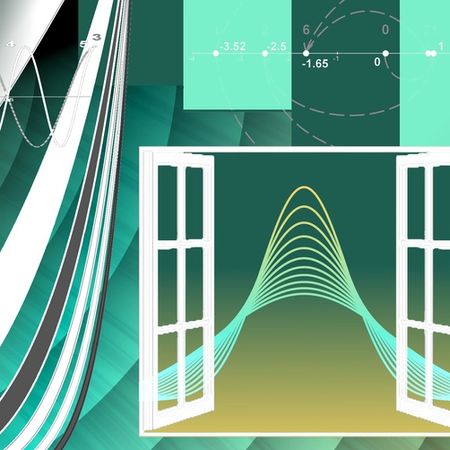
We mentioned one input item already, which is the “average.” We can change the “ingredient” average and produce different bell curves. Here are some examples of the bell curve where we only change one ingredient, the “average.” Notice this simply shifts the curve to the left or right.

A second ingredient is the standard deviation which measures variability. Now, let’s view examples of the curve where we only change the standard deviation.

Observe that when we change the standard deviation, it has the effect of “pushing down and squeezing out” the curve.

Think for a moment the change in the curve if we change both the average and the standard deviation at the same time. Here are some sample curves when we change both the average and the standard deviation.

These curves are pretty, wouldn’t you agree?

We can use the normal curve in many ways to solve problems in statistics. This occurs when we have a process that we repeat a large number of times. Then the distribution of the results leans toward a normal distribution.

For example, if we flip a two-sided fair coin, the probabilities we flip a head or a tail are both 50%. Certainly, flipping a coin does not produce a normal distribution. If we flip 1,000 coins, we expect to get 500 heads. But, if we flipped 1,000 coins, how many heads would we actually get? Maybe we get exactly 500. However, it is more accurate to say we would get “about 500.” How could we quantify what we expect for the results?

Let’s say you performed this experiment 10,000 times, recorded the number of heads each time and graphed the outcomes. What would the graph resemble? The graph would resemble a normal curve. The more times we repeat the experiment, the closer the result would lean towards a perfect normal curve.

I mentioned two of the ingredients to the normal curve, the average, or mean, and the standard deviation. Another ingredient to produce the normal curve is $e$. As we will witness often in this book, $e$ commonly appears when we take the limit of some process. Here, we are flipping 1,000 coins. The more times we flip 1,000 coins, the closer we get to a result that has a base e. Isn’t it fascinating that this rather strange number has this unique characteristic?

A fourth ingredient to our recipe is $\pi$. Are you surprised $\pi$ is included in this recipe? I am. What we are saying is that the number of heads when we flip a coin many times is somehow related to a circle. If it wasn’t, then $\pi$ would not be in this recipe.

We do have a “pure vanilla” version for our recipe of a normal curve when the average is 0 and the standard deviation is 1. We call this the standard normal distribution. This “pure vanilla” version isn’t quite as messy and is worth reviewing.

Here is the formula for the normal distribution if the average is 0 and the standard deviation is 1:

$$y = \frac{1}{\sqrt{2\pi}}e^{- \frac{1}{2}x^{2}}$$

Notice this is similar to the “natural exponential function” we just reviewed but with 3 changes. First, there is the constant factor in front that contains $\pi$. The second change is the exponent has a $-\frac{1}{2}$ factor in front. The third change is we square $x$.

Observe that if we want to investigate why $\pi$ appears in this formula, the mystery deepens because we must identify why $\sqrt{2\pi}$ appears, not just $\pi$. I usually don’t consider the natural exponential function and the normal distribution as related. However, with only 3 changes, we can change the simple natural exponential function and create the normal distribution. I’ve worked with the exponential and the normal distribution often in my career, but it’s only recently that I realized how closely related these two functions are. This illustrates how easy it is to get lost in the weeds and miss the big connections.

History 2

By the way, have you ever wondered how we got this normal distribution? As usual, it was a team effort in math. But in 1809, most of the credit was given to Carl Friedrich Gauss (1777−1855), one of the most brilliant mathematicians of all time. In fact, another name for the normal distribution is the Gaussian distribution.

However, the roots go back further to de Moivre, who in 1733 identified what we just discussed. If you flip a coin enough times, the number of heads will drift towards a normal distribution. That means if we flip a coin 1000 times, we can model the number of heads by using $e$ and $\pi$.

But there was another important person before de Moivre. Before de Moivre used the normal distribution to model coin flips, Jacob Bernoulli explained the law of large numbers. Basically, this law tells us there are patterns that we can predict if we perform an experiment a large number of times. This is what Bernoulli used in the continuous interest compounding experiment we discussed earlier in this section.

In short, Bernoulli discovered the number $e$, de Moivre connected flipping coins a large number of times to a bell curve, and Gauss put it all together and made it official. All these interesting stories provided a foundation for not only pure math but applied math, with applications to areas such as actuarial science and engineering.

If you are interested in why $\pi$ appears in the normal distribution, there are many YouTube videos that explain it well.

We have completed our journey through the foundation of math by using numbers. We’ve travelled far into the number line. We’ve identified three interesting points on the number line: $\sqrt{2}, \pi,$ and $e$. We’ve identified how $\pi$ is connected to a circle. As we journey into Foundation 2, we will understand how dimensions are important. In doing so, we will dig deeper into $\pi$ and the circle to discover more treasures.